Ever wondered how your computer or your phone displays the current date and time accurately? What keeps all the devices in the world (and in space) in agreement on what time it is? What makes applications that require precise timing possible?

In this article, I will explain some of the challenges with time synchronization and explore two of the most popular protocols that devices use to keep their time in sync: the Network Time Protocol (NTP) and the Precision Time Protocol (PTP).

What is time?

It wouldn’t be a good article about time synchronization without spending a few words about time. We all have an intuitive concept of time since childhood, but stating precisely what ‘time’ is can be quite a challenge. I’m going to give you my idea of it.

Here is a simple definition to start with: time is how we measure changes. If the objects in the universe didn’t change and appeared to be fixed, without ever moving or mutating, I think we could all agree that time wouldn’t be flowing. Here by ‘change’ I mean any kind of change: from objects falling or changing shape, to light diffusing through space, or our memories building up in our mind.

This definition may be a starting point but does not capture all we know about time. Something that it does not capture is our concept of past, present, and future. From our day-to-day experience, we know in fact that an apple would fall off the tree due to gravity, under the normal flow of time. If we observed an apple rising from the ground, attaching itself to the tree (without the action of external forces), we could perhaps agree that what we’re observing is time flowing backward. And yet, both the apple falling off the tree and the apple rising from the ground are two valid changes from an initial state. This is where causality comes into place: time flows in such a way that the cause must precede the effect.

We can now refine our definition of time as an ordered sequence of changes, where each change is linked to the previous one by causality.

How do we measure time?

Now we have a more precise definition of time, but we still don’t have enough tools to define what is a second, an hour, or a day. This is where things get more complicated.

If we look at the definition of ‘second’ from the international standard, we can see that it is currently defined from the emission frequency of caesium-133 (¹³³Cs) atoms. If you irradiate caesium-133 atoms with some light having sufficient energy, the atoms will absorb the light, get excited, and release the energy back in the form of light at a specific frequency. That frequency of emission is defined as 9192631770 Hz, and the second is defined as the inverse of that frequency. This definition is known as the caesium standard.

Here’s a problem to think about: how do we know that a caesium-133 atom, after getting excited, really emits light at a fixed frequency? The definition of second is implying that the frequency is constant and the same all over the world, but how do we know it’s really the case? This assumption is supported by quantum physics, according to which atoms can only transition between discrete (quantified) energy states. When an atom gets excited, it transitions from an energy state $E_1$ to an energy state $E_2$. Atoms like to be in the lowest energy state, so the atom will not stay in the state $E_2$ for long, and will want to go back to $E_1$. When doing that, it will release an amount of energy of exactly $E_2 - E_1$ in the form of a photon. According to the Planck formula, the photon will have frequency $f = (E_2 - E_1) / h$ where $h$ is the Planck constant. Because the energy levels are fixed, the resulting emission frequency is fixed as well.

By the way, this process of absorption and emission of photons is the same process that causes fluorescence.

Assuming that caesium-133 atoms emit light at a single, fixed frequency, we can now build extremely accurate caesium atomic clocks and measure spans of time with them. Existing caesium atomic clocks are estimated to be so precise that they may lose one second every 100 million years.

The same approach can be applied to other substances as well: atomic clocks have been constructed using rubidium (Rb), strontium (Sr), hydrogen (H), krypton (Kr), ammonia (NH₃), ytterbium (Yb), each having its own emission frequency, and their own accuracy. The most accurate clock ever built is a strontium clock which may lose one second every 15 billion years.

Time dilation

If we have two atomic clocks and we let them run for a while, will they show the same time? This might sound like a rhetorical question: we just established that the frequencies of emission of atoms are fixed, so why would two identical atomic clocks ever get out of sync? Well, as a matter of fact, two identical atomic clocks may get out of sync, and this problem is not due to the clocks, but with time itself: it appears that time does not always flow in the same way everywhere.

Many experiments have shown this effect on our planet, the most famous one probably being the Hafele-Keating experiment. In this experiment, a set of caesium clocks was placed on an airplane flying around the world west-to-east, another set was placed on an airplane flying east-to-west, and another set remained on ground. The 3 sets of clocks, which were initially in sync before the planes took off, were showing different times once reunited after the trip. This experiment and similar ones have been repeated and refined multiple times, and they all showed consistent results.

These effects were due to time dilation, and the results were consistent with the predictions of special relativity and general relativity.

Time dilation due to special relativity

Special relativity predicts that if two clocks are moving with two different velocities, they are going to measure different spans of time.

Special relativity is based on two principles:

• the speed of light is constant;
• there are no privileged reference frames.

To understand how these principles affect the flow of time, it’s best to look at an example: imagine that a passenger is sitting on a train with a laser and a mirror in front of them. Another person is standing on the ground next to the railroad and observing the train passing. The passenger points the laser perpendicular to the mirror and turns it on.

What the passenger will observe is the beam of light from the laser to hit the mirror and come back in a straight line:

From the observer perspective, however, things are quite different. Because the train is moving relative to the observer, the beam looks like it’s taking a different, slightly longer path:

If both the passenger and the observer measure how long it took for the light beam to hit back at the source, and if the principles of special relativity hold, then the two persons will record different measurements. If the speed of light is constant, and there is no privileged reference frame, then the speed of light $c$ must be the same in both reference frames. From the passenger’s perspective, the beam has traveled a distance of $2 L$, taking a time $2 L / c$. From the observer’s perspective, the beam has traveled a longer distance $2 M$, with $M > L$, taking a longer time $2 M / c$.

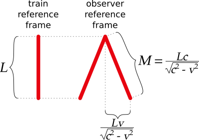
How can we reconcile these counterintuitive measurements? Special relativity does it is by stating that time flows differently in the two reference frames. Time runs “slower” inside the train and runs “faster” for the observer. One consequence of that is that the passenger ages less than the observer.

Time dilation due to special relativity is not easily detectable in our day-to-day life, but it can still cause problems with high-precision clocks. This time dilation may in fact cause clock drifts in the order of hundreds of nanoseconds per day.

Time dilation due to general relativity

Experimental data shows that clocks in a gravitational field do not follow (solely) the rules of special relativity. This does not mean that special relativity is wrong, but it’s a sign that it is incomplete. This is where general relativity comes into play. In general relativity, gravity is not seen as a force, like in classical physics, but rather as a deformation of spacetime. All objects that have mass bend spacetime, and the path of objects traveling through spacetime is affected by its curvature.

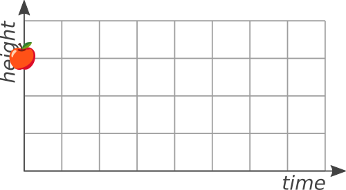
An apple falling from a tree is not going towards the ground because there’s a force “pushing” it down, but rather because that’s the shortest path in spacetime (a straight line in bent spacetime).

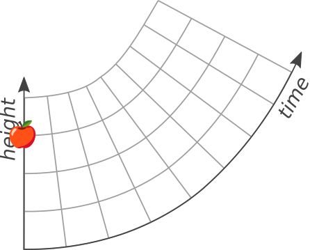
The larger the mass of objects, the larger the curvature of spacetime they produce. Time flows “slower” near large masses, and “faster” away from it. Interesting facts: people on a mountain age faster than people on the sea level, and it has been calculated that the core of the Earth is 2.5 years younger than the crust.

The time dilation caused by gravity on the surface of the Earth may amount to clock drifts in the order of hundreds of nanoseconds per day, just like special relativity.

Can we actually synchronize clocks?

Given what we have seen about time dilation, and that we may experience time differently, does it even make sense to talk about time synchronization? Can we agree on time if time flows differently for us?

The short answer is yes: the trick is to restrict our view to a closed system, like the surface of our planet. If we place some clocks scattered across the system, they will almost certainly experience different flows of time, due to different velocities, different altitudes, and other time dilation phenomena. We cannot make those clocks agree on how much time has passed since a specific event; what we can do is aggregate all the time measurements from the clocks and average them out. This way we end up with a value that is representative of how much time has passed on the entire system—in other words, we get an “overall time” for the system.

Very often, the system that we consider is not restricted to just the surface of our planet, but involves the Sun, and sometimes the moon as well. In fact, what we call one year is roughly the time it takes for the Earth to complete an orbit around the Sun; one day is roughly the time it takes for the Earth to spin around itself once and face the Sun in the same position again. Including the Sun (or the moon) in our time measurements is complicated: in part this complexity comes from the fact that precise measurements of the Earth’s position are difficult, and in part from the fact that the Earth’s rotation is not regular, not fully predictable, and it’s slowing down. It’s worth noting that climate and geological events affect the Earth’s rotation in a measurable way, and such events are very hard to model accurately.

What is important to understand here is that the word ‘time’ is often used to mean different things. Depending on how we measure it, we can end up with different definitions of time. To avoid ambiguity, I will classify ‘time’ into two big categories:

• Elapsed time: this is the time measured directly by a clock, without using any extra information about the system where the clock lies into or about other clocks.

  We can use elapsed time to measure durations, latencies, frequencies, as well as lengths.

• Coordinated time: this is the time measured by using a clock, paired with information about the system where it’s located (like position, velocity, and gravity), and/or information from other clocks.

  This notion of time is mostly useful for coordinating events across the system. Some practical examples: scheduling the execution of tasks in the future, checking the expiration of certificates, real-time communication.

Time standards

Over the centuries several time standards have been introduced to measure coordinated time. Nowadays there are three major standards in use: TAI, UTC, and GNSS. Let’s take a brief look at them.

TAI

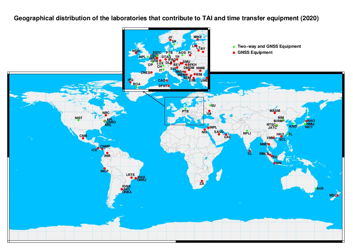
International Atomic Time (TAI) is based on the weighted average of the elapsed time measured by several atomic clocks spread across the world. The more a clock in TAI is precise, the more it contributes to the weighted average. The fact that the clocks are spread in multiple locations, and the use of an average, mitigates relativistic effects and yields a value that we can think of as the overall time flow experienced by the surface of the Earth.

Note that the calculations for TAI does not include the Earth’s position with respect to the Sun.

UTC

Coordinated Universal Time (UTC) is built upon TAI. UTC, unlike TAI, is periodically adjusted to synchronize it with the Earth’s rotation around itself and the Sun. The goal is to make sure that 24 UTC hours are equivalent to a solar day (within a certain degree of precision). Because, as explained earlier, the Earth’s rotation is irregular, not fully predictable, and slowing down, periodic adjustments have to be made to UTC at irregular intervals.

The adjustments are performed by inserting leap seconds: these are extra seconds that are added to the UTC time to “slow down” the UTC time flow and keep it in sync with Earth’s rotation. On days when a leap second is inserted, UTC clocks go from 23:59:59 to 23:59:60.

It’s worth noting that the practice of inserting leap seconds is most likely going to be discontinued in the future. The main reason is that leap seconds have been the source of complexity and bugs in computer systems, and the benefit-to-pain ratio of leap seconds is not considered high enough to keep adding them. If leap seconds are discontinued, UTC will become effectively equivalent to TAI, with an offset: UTC will always differ from TAI by a few seconds, but this difference will always be constant, if no more leap seconds are inserted.

GNSS

Global Navigation Satellite System (GNSS) is based on a mix of accurate atomic clocks on ground and less accurate atomic clocks on artificial satellites orbiting around the Earth. The clocks on the satellites, being less accurate and subject to a variety of relativistic effects, are updated about twice a day from ground stations to correct clock drifts. Nowadays there are several implementations of GNSS around the world, including:

• the United States’ Global Positioning System (GPS);
• the European Galileo system;
• China’s BeiDou (BDS);
• the Russian GLONASS.

When GPS was launched, it was synchronized with UTC, however GPS, unlike UTC, is not adjusted to follow the Earth’s rotation, and due to that, GPS today differs from UTC by 18 seconds (because 18 leap seconds have been inserted since GPS was launched in 1980). BeiDou also does not implement leap seconds. GPS and BeiDou are therefore compatible with TAI.

Other GNSS systems like Galileo and GLONASS do implement leap seconds and are therefore compatible with UTC.

Time synchronization protocols

Dealing with coordinated time is not trivial. Different ways to deal with relativistic effects and Earth’s irregular rotation result in different time standards that are not always immediately compatible with each other. Nonetheless, once we agree on a well-defined time standard, we have a way to ask the question “what time is it?” and receive an accurate answer all around the world (within a certain degree of precision).

Let’s now take a look at how computers on a network can obtain an accurate value for the coordinated time given by a time standard. I will describe two popular protocols: NTP and PTP. The two are using similar algorithms, but offer different precision: milliseconds (NTP) and nanoseconds (PTP). Both use UDP/IP as the transport protocol.

Network Time Protocol (NTP)

The way time synchronization works with NTP is the following: a computer that wants to synchronize its time periodically queries an NTP server (or multiple servers) to get the current coordinated time. The server that provides the current coordinated time may have obtained the time from an accurate source clock connected to the server (like an atomic clock synchronized with TAI or UTC, or a GNSS receiver), or from a previous synchronization from another NTP server.

To record how “fresh” the coordinated time from an NTP server is (how distant the NTP server is from the source clock), NTP has a concept of stratum: this is a number that indicates the number of ‘hops’ from the accurate clock source:

• stratum 0 is used to indicate an accurate clock;
• stratum 1 is a server that is directly connected to a stratum 0 clock;
• stratum 2 is a server that is synchronized from a stratum 1 server;
• stratum 3 is a server that is synchronized from a stratum 2 server;
• and so on…

The maximum stratum allowed is 15. There’s also a special stratum 16: this is not a real stratum, but a special value used by clients to indicate that time synchronization is not happening (most likely because the NTP servers are unreachable).

The major problem with synchronizing time over a network is latency. Networks can be composed of multiple links, some of which may be slow or overloaded. Simply requesting the current time from an NTP server without taking latency into account would lead to an imprecise response. Here is how NTP deals with this problem:

1. The NTP client sends a request via a UDP packet to an NTP server. The packet includes an originate timestamp $t_0$ that indicates the local time of the client when the packet was sent.
2. The NTP server receives the request and records the receive timestamp $t_1$, which indicates the local time of the server when the request was received.
3. The NTP server processes the request, prepares a response, and records the transmit timestamp $t_2$, which indicates the local time of the server when the response was sent. The timestamps $t_0$, $t_1$ and $t_2$ are all included in the response.
4. The NTP client receives the response and records the timestamp $t_3$, which indicates the local time of the client when the response was received.

Our goal is now to calculate an estimate for the network latency and processing delay and use that information to calculate, in the most accurate way possible, the offset between the NTP client clock and the NTP server clock.

The difference $t_3 - t_0$ is the duration of the overall exchange. The difference $t_2 - t_1$ is the duration of the NTP server processing delay. If we subtract these two durations, we get the total network latency experienced, also known as round-trip delay:

$$\delta = (t_3 - t_0) - (t_2 - t_1)$$

If we assume that the transmit delay and the receive delay are the same, then $\delta / 2$ is the average network latency (this assumption may not be true in a general network, but that’s the assumption that NTP makes).

Under this assumption, the time $t_0 + \delta/2$ is the time on the client’s clock that corresponds to $t_1$ on the server’s clock. Similarly, $t_3 - \delta/2$ on the client’s clock corresponds to $t_2$ on the server’s clock. These correspondences let us calculate two estimates for the offset between the client’s clock and the server’s clock:

$$\begin{align*} \theta_1 & = t_1 - (t_0 + \delta/2) \\ \theta_2 & = t_2 - (t_3 - \delta/2) \end{align*}$$

We can now calculate the client-server offset $\theta$ as an average of those two estimates:

$$\begin{align*} \theta & = \frac{\theta_1 + \theta_2}2 \\ & = \frac{t_1 - (t_0 + \delta/2) + t_2 - (t_3 - \delta/2)}2 \\ & = \frac{t_1 - t_0 - \delta/2 + t_2 - t_3 + \delta/2}2 \\ & = \frac{(t_1 - t_0) + (t_2 - t_3)}2 \\ \end{align*}$$

Note that the offset $\theta$ may be a positive duration (meaning that the client clock is in the past), a negative duration (meaning that the client clock is in the future) or zero (meaning that the client clock agrees with the server clock, which is unlikely).

After calculating the offset $\theta$, the client can update its local clock by shifting it by $\theta$ and from that point the client will be in sync with the server (within a certain degree of precision).

Once the synchronization is done, it is expected that the client’s clock will start drifting away from the server’s clock. This may happen due to relativistic effects and more importantly because often clients do not use high-precision clocks. For this reason, it is important that NTP clients synchronize their time periodically. Usually NTP clients start by synchronizing time every minute or so when they are started, and then progressively slow down until they synchronize time once every half an hour or every hour.

There are some drawbacks with this synchronization method:

• The request and response delays may not be perfectly symmetric, resulting in inaccuracies in the calculations of the offset $\theta$. Network instabilities, packet retransmissions, change of routes, queuing may all cause unpredictable and inconsistent delays.
• The timestamps $t_1$ and $t_3$ must be set as soon as possible (as soon as the packets are received), and similarly $t_0$ and $t_2$ must be set as late as possible. Because NTP is implemented at the software level, there may be non-negligible delays in acquiring and recording these timestamps. These delays may be exacerbated if the NTP implementation is not very performant, or if the client or server are under high load.
• Errors propagate and add up when increasing the number of strata.

For all these reasons, NTP clients do not synchronize time just from a single NTP server, but from multiple ones. NTP clients take into account the round-trip delays, stratum, and jitter (the variance in round-trip delays) to decide the best NTP server to get their time from. Under ideal network conditions, an NTP client will always prefer a server with a low stratum. However, an NTP client may prefer an NTP server with high stratum and more reliable connectivity over an NTP server with low stratum but a very unstable network connection.

The precision offered by NTP is in the order of a few milliseconds.

Precision Time Protocol (PTP)

PTP is a time synchronization protocol for applications that require more accuracy than the one provided by NTP. The main differences between PTP and NTP are:

• Precision: NTP offers millisecond precision, while PTP offers nanosecond precision.
• Time standard: NTP transmits UTC time, while PTP transmits TAI time and the difference between TAI and UTC.
• Scope: NTP is designed to be used over large networks, including the internet, while PTP is designed to be used in local area networks.
• Implementation: NTP is mainly software based, while PTP can be implemented both via software and on specialized hardware. The use of specialized hardware considerably reduces delays and jitter introduced by software.

• Hierarchy: NTP can support a complex hierarchy of NTP servers, organized via strata. While PTP does not put a limitation on the number of nodes involved, the hierarchy is usually only composed of master clocks (the source of time information) and slave clocks (the receivers of time information). Sometimes boundary clocks are used to relay time information to network segments that are unreachable by the master clocks.
• Clock selection: in NTP, clients select the best NTP server to use based on the NTP server clock quality and the network connection quality. In PTP, slaves do not select the best master clock to use. Instead, master clocks perform a selection between themselves using a method called best master clock algorithm. This algorithm takes into account the clock’s quality and input from system administrators, and does not factor network quality at all. The master clock selected by the algorithm is called grandmaster clock.

• Algorithm: in NTP, clients poll the time information from servers periodically and calculate the clock offset using the algorithm described above (based on the timestamps $t_0$, $t_1$, $t_2$ and $t_3$). With PTP, the algorithm used by slaves to calculate the offset from the grandmaster clock is somewhat similar to the one used in NTP, but the order of operations is different:

  1. the grandmaster periodically broadcasts its time information $T_0$ over the network;
  2. each slave records the time $T_1$ when the broadcasted time was received;
  3. each slave sends a packet to the grandmaster at time $T_2$;
  4. the grandmaster receives the packet at time $T_3$ and sends that value back to the slave.

  The average network delay can be calculated as $\delta = ((T_3 - T_0) - (T_2 - T_1)) / 2$. The clock offset can be calculated as $\theta = ((T_1 - T_0) + (T_2 - T_3)) / 2$.

Summary

• Synchronizing time across a computer network is not an easy task, and first of all requires agreeing on a definition of ‘time’ and on a time standard.
• Relativistic effects make it so that time may not flow at the same speed all over the globe, and this means that time has to be measured and aggregated across the planet in order to get a suitable value that can be agreed on.
• Atomic clocks and GNSS are the clock sources used for most applications nowadays.
• NTP is a time synchronization protocol that can be used on large and distributed networks like the internet and provides millisecond precision.
• PTP is a time synchronization protocol for local area networks and provides nanosecond precision.