Those of you who know what public-key cryptography is may have already heard of ECC, ECDH or ECDSA. The first is an acronym for Elliptic Curve Cryptography, the others are names for algorithms based on it.

Today, we can find elliptic curves cryptosystems in TLS, PGP and SSH, which are just three of the main technologies on which the modern web and IT world are based. Not to mention Bitcoin and other cryptocurrencies.

Before ECC become popular, almost all public-key algorithms were based on RSA, DSA, and DH, alternative cryptosystems based on modular arithmetic. RSA and friends are still very important today, and often are used alongside ECC. However, while the magic behind RSA and friends can be easily explained, is widely understood, and rough implementations can be written quite easily, the foundations of ECC are still a mystery to most.

With a series of blog posts I’m going to give you a gentle introduction to the world of elliptic curve cryptography. My aim is not to provide a complete and detailed guide to ECC (the web is full of information on the subject), but to provide a simple overview of what ECC is and why it is considered secure, without losing time on long mathematical proofs or boring implementation details. I will also give helpful examples together with visual interactive tools and scripts to play with.

Specifically, here are the topics I’ll touch:

1. Elliptic curves over real numbers and the group law (covered in this blog post)
2. Elliptic curves over finite fields and the discrete logarithm problem
3. Key pair generation and two ECC algorithms: ECDH and ECDSA
4. Algorithms for breaking ECC security, and a comparison with RSA

In order to understand what’s written here, you’ll need to know some basic stuff of set theory, geometry and modular arithmetic, and have familiarity with symmetric and asymmetric cryptography. Lastly, you need to have a clear idea of what an “easy” problem is, what a “hard” problem is, and their roles in cryptography.

Ready? Let’s start!

Elliptic Curves

First of all: what is an elliptic curve? Wolfram MathWorld gives an excellent and complete definition. But for our aims, an elliptic curve will simply be the set of points described by the equation: $$y^2 = x^3 + ax + b$$

where $4a^3 + 27b^2 \ne 0$ (this is required to exclude singular curves). The equation above is what is called Weierstrass normal form for elliptic curves.

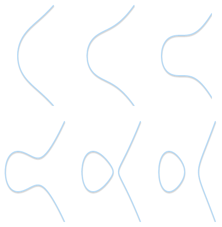
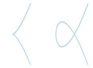
Depending on the value of $a$ and $b$, elliptic curves may assume different shapes on the plane. As it can be easily seen and verified, elliptic curves are symmetric about the $x$-axis.

For our aims, we will also need a point at infinity (also known as ideal point) to be part of our curve. From now on, we will denote our point at infinity with the symbol 0 (zero).

If we want to explicitly take into account the point at infinity, we can refine our definition of elliptic curve as follows: $$\left\{ (x, y) \in \mathbb{R}^2\ |\ y^2 = x^3 + ax + b,\ 4 a^3 + 27 b^2 \ne 0 \right\}\ \cup\ \left\{ 0 \right\}$$

Groups

A group in mathematics is a set for which we have defined a binary operation that we call “addition” and indicate with the symbol +. In order for the set $\mathbb{G}$ to be a group, addition must defined so that it respects the following four properties:

1. closure: if $a$ and $b$ are members of $\mathbb{G}$, then $a + b$ is a member of $\mathbb{G}$;
2. associativity: $(a + b) + c = a + (b + c)$;
3. there exists an identity element 0 such that $a + 0 = 0 + a = a$;
4. every element has an inverse, that is: for every $a$ there exists $b$ such that $a + b = 0$.

If we add a fifth requirement:

5. commutativity: $a + b = b + a$,

then the group is called abelian group.

With the usual notion of addition, the set of integer numbers $\mathbb{Z}$ is a group (moreover, it’s an abelian group). The set of natural numbers $\mathbb{N}$ however is not a group, as the fourth property can’t be satisfied.

Groups are nice because, if we can demonstrate that those four properties hold, we get some other properties for free. For example: the identity element is unique; also the inverses are unique, that is: for every $a$ there exists only one $b$ such that $a + b = 0$ (and we can write $b$ as $-a$). Either directly or indirectly, these and other facts about groups will be very important for us later.

The group law for elliptic curves

We can define a group over elliptic curves. Specifically:

• the elements of the group are the points of an elliptic curve;
• the identity element is the point at infinity 0;
• the inverse of a point $P$ is the one symmetric about the $x$-axis;
• addition is given by the following rule: given three aligned, non-zero points $P$, $Q$ and $R$, their sum is $P + Q + R = 0$.

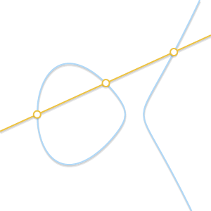
Note that with the last rule, we only require three aligned points, and three points are aligned without respect to order. This means that, if $P$, $Q$ and $R$ are aligned, then $P + (Q + R) = Q + (P + R) = R + (P + Q) = \cdots = 0$. This way, we have intuitively proved that our + operator is both associative and commutative: we are in an abelian group.

So far, so great. But how do we actually compute the sum of two arbitrary points?

Geometric addition

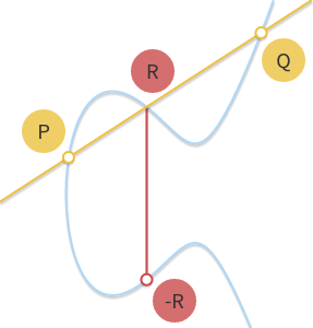
Thanks to the fact that we are in an abelian group, we can write $P + Q + R = 0$ as $P + Q = -R$. This equation, in this form, lets us derive a geometric method to compute the sum between two points $P$ and $Q$: if we draw a line passing through $P$ and $Q$, this line will intersect a third point on the curve, $R$ (this is implied by the fact that $P$, $Q$ and $R$ are aligned). If we take the inverse of this point, $-R$, we have found the result of $P + Q$.

This geometric method works but needs some refinement. Particularly, we need to answer a few questions:

• What if $P = 0$ or $Q = 0$? Certainly, we can’t draw any line (0 is not on the $xy$-plane). But given that we have defined 0 as the identity element, $P + 0 = P$ and $0 + Q = Q$, for any $P$ and for any $Q$.
• What if $P = -Q$? In this case, the line going through the two points is vertical, and does not intersect any third point. But if $P$ is the inverse of $Q$, then we have $P + Q = P + (-P) = 0$ from the definition of inverse.
• What if $P = Q$? In this case, there are infinitely many lines passing through the point. Here things start getting a bit more complicated. But consider a point $Q’ \ne P$. What happens if we make $Q’$ approach $P$, getting closer and closer to it?
  

  

As $Q’$ tends towards $P$, the line passing through $P$ and $Q’$ becomes tangent to the curve. In the light of this we can say that $P + P = -R$, where $R$ is the point of intersection between the curve and the line tangent to the curve in $P$. * What if $P \ne Q$, but there is no third point $R$? We are in a case very similar to the previous one. In fact, we are in the case where the line passing through $P$ and $Q$ is tangent to the curve.

Let’s assume that $P$ is the tangency point. In the previous case, we would have written $P + P = -Q$. That equation now becomes $P + Q = -P$. If, on the other hand, $Q$ were the tangency point, the correct equation would have been $P + Q = -Q$.

The geometric method is now complete and covers all cases. With a pencil and a ruler we are able to perform addition involving every point of any elliptic curve. If you want to try, take a look at the HTML5/JavaScript visual tool I’ve built for computing sums on elliptic curves!

Algebraic addition

If we want a computer to perform point addition, we need to turn the geometric method into an algebraic method. Transforming the rules described above into a set of equations may seem straightforward, but actually it can be really tedious because it requires solving cubic equations. For this reason, here I will report only the results.

First, let’s get get rid of the most annoying corner cases. We already know that $P + (-P) = 0$, and we also know that $P + 0 = 0 + P = P$. So, in our equations, we will avoid these two cases and we will only consider two non-zero, non-symmetric points $P = (x_P, y_P)$ and $Q = (x_Q, y_Q)$.

If $P$ and $Q$ are distinct ($x_P \ne x_Q$), the line through them has slope: $$m = \frac{y_P - y_Q}{x_P - x_Q}$$

The intersection of this line with the elliptic curve is a third point $R = (x_R, y_R)$: $$\begin{align*} x_R & = m^2 - x_P - x_Q \\ y_R & = y_P + m(x_R - x_P) \end{align*}$$

or, equivalently: $$y_R = y_Q + m(x_R - x_Q)$$

Hence $(x_P, y_P) + (x_Q, y_Q) = (x_R, -y_R)$ (pay attention at the signs and remember that $P + Q = -R$).

If we wanted to check whether this result is right, we would have had to check whether $R$ belongs to the curve and whether $P$, $Q$ and $R$ are aligned. Checking whether the points are aligned is trivial, checking that $R$ belongs to the curve is not, as we would need to solve a cubic equation, which is not fun at all.

Instead, let’s play with an example: according to our visual tool, given $P = (1, 2)$ and $Q = (3, 4)$ over the curve $y^2 = x^3 - 7x + 10$, their sum is $P + Q = -R = (-3, 2)$. Let’s see if our equations agree: $$\begin{align*} m & = \frac{y_P - y_Q}{x_P - x_Q} = \frac{2 - 4}{1 - 3} = 1 \\ x_R & = m^2 - x_P - x_Q = 1^2 - 1 - 3 = -3 \\ y_R & = y_P + m(x_R - x_P) = 2 + 1 \cdot (-3 - 1) = -2 \\ & = y_Q + m(x_R - x_Q) = 4 + 1 \cdot (-3 - 3) = -2 \end{align*}$$

Yes, this is correct!

Note that these equations work even if one of $P$ or $Q$ is a tangency point. Let’s try with $P = (-1, 4)$ and $Q = (1, 2)$. $$\begin{align*} m & = \frac{y_P - y_Q}{x_P - x_Q} = \frac{4 - 2}{-1 - 1} = -1 \\ x_R & = m^2 - x_P - x_Q = (-1)^2 - (-1) - 1 = 1 \\ y_R & = y_P + m(x_R - x_P) = 4 + -1 \cdot (1 - (-1)) = 2 \end{align*}$$

We get the result $P + Q = (1, -2)$, which is the same result given by the visual tool.

The case $P = Q$ needs to be treated a bit differently: the equations for $x_R$ and $y_R$ are the same, but given that $x_P = x_Q$, we must use a different equation for the slope: $$m = \frac{3 x_P^2 + a}{2 y_P}$$

Note that, as we would expect, this expression for $m$ is the first derivative of: $$y_P = \pm \sqrt{x_P^3 + ax_P + b}$$

To prove the validity of this result it is enough to check that $R$ belongs to the curve and that the line passing through $P$ and $R$ has only two intersections with the curve. But again, we don’t prove this fact, and instead try with an example: $P = Q = (1, 2)$. $$\begin{align*} m & = \frac{3x_P^2 + a}{2 y_P} = \frac{3 \cdot 1^2 - 7}{2 \cdot 2} = -1 \\ x_R & = m^2 - x_P - x_Q = (-1)^2 - 1 - 1 = -1 \\ y_R & = y_P + m(x_R - x_P) = 2 + (-1) \cdot (-1 - 1) = 4 \end{align*}$$

Which gives us $P + P = -R = (-1, -4)$. Correct!

Although the procedure to derive them can be really tedious, our equations are pretty compact. This is thanks to Weierstrass normal form: without it, these equations could have been really long and complicated!

Scalar multiplication

Other than addition, we can define another operation: scalar multiplication, that is: $$nP = \underbrace{P + P + \cdots + P}_{n\ \text{times}}$$

where $n$ is a natural number. I’ve written a visual tool for scalar multiplication too, if you want to play with that.

Written in that form, it may seem that computing $nP$ requires $n$ additions. If $n$ has $k$ binary digits, then our algorithm would be $O(2^k)$, which is not really good. But there exist faster algorithms.

One of them is the double and add algorithm. Its principle of operation can be better explained with an example. Take $n = 151$. Its binary representation is $10010111_2$. This binary representation can be turned into a sum of powers of two: $$\begin{align*} 151 & = 1 \cdot 2^7 + 0 \cdot 2^6 + 0 \cdot 2^5 + 1 \cdot 2^4 + 0 \cdot 2^3 + 1 \cdot 2^2 + 1 \cdot 2^1 + 1 \cdot 2^0 \\ & = 2^7 + 2^4 + 2^2 + 2^1 + 2^0 \end{align*}$$

(We have taken each binary digit of $n$ and multiplied it by a power of two.)

In view of this, we can write: $$151 \cdot P = 2^7 P + 2^4 P + 2^2 P + 2^1 P + 2^0 P$$

What the double and add algorithm tells us to do is:

• Take $P$.
• Double it, so that we get $2P$.
• Add $2P$ to $P$ (in order to get the result of $2^1P + 2^0P$).
• Double $2P$, so that we get $2^2P$.
• Add it to our result (so that we get $2^2P + 2^1P + 2^0P$).
• Double $2^2P$ to get $2^3P$.
• Don’t perform any addition involving $2^3P$.
• Double $2^3P$ to get $2^4P$.
• Add it to our result (so that we get $2^4P + 2^2P + 2^1P + 2^0P$).
• …

In the end, we can compute $151 \cdot P$ performing just seven doublings and four additions.

If this is not clear enough, here’s a Python script that implements the algorithm:

def bits(n):
    """
    Generates the binary digits of n, starting
    from the least significant bit.

    bits(151) -> 1, 1, 1, 0, 1, 0, 0, 1
    """
    while n:
        yield n & 1
        n >>= 1

def double_and_add(n, x):
    """
    Returns the result of n * x, computed using
    the double and add algorithm.
    """
    result = 0
    addend = x

    for bit in bits(n):
        if bit == 1:
            result += addend
        addend *= 2

    return result

If doubling and adding are both $O(1)$ operations, then this algorithm is $O(\log n)$ (or $O(k)$ if we consider the bit length), which is pretty good. Surely much better than the initial $O(n)$ algorithm!

Logarithm

Given $n$ and $P$, we now have at least one polynomial time algorithm for computing $Q = nP$. But what about the other way round? What if we know $Q$ and $P$ and need to find out $n$? This problem is known as the logarithm problem. We call it “logarithm” instead of “division” for conformity with other cryptosystems (where instead of multiplication we have exponentiation).

I don’t know of any “easy” algorithm for the logarithm problem, however playing with multiplication it’s easy to see some patterns. For example, take the curve $y^2 = x^3 - 3x + 1$ and the point $P = (0, 1)$. We can immediately verify that, if $n$ is odd, $nP$ is on the curve on the left semiplane; if $n$ is even, $nP$ is on the curve on the right semiplane. If we experimented more, we could probably find more patterns that eventually could lead us to write an algorithm for computing the logarithm on that curve efficiently.

But there’s a variant of the logarithm problem: the discrete logarithm problem. As we will see in the next post, if we reduce the domain of our elliptic curves, scalar multiplication remains “easy”, while the discrete logarithm becomes a “hard” problem. This duality is the key brick of elliptic curve cryptography.

See you next week

That’s all for today, I hope you enjoyed this post! Next week we will discover finite fields and the discrete logarithm problem, along with examples and tools to play with. If this stuff sounds interesting to you, then stay tuned!

Read the next post of the series »